Kevin Chen Purdue CS ’29
Portfolio Vision Pick and Place Robot
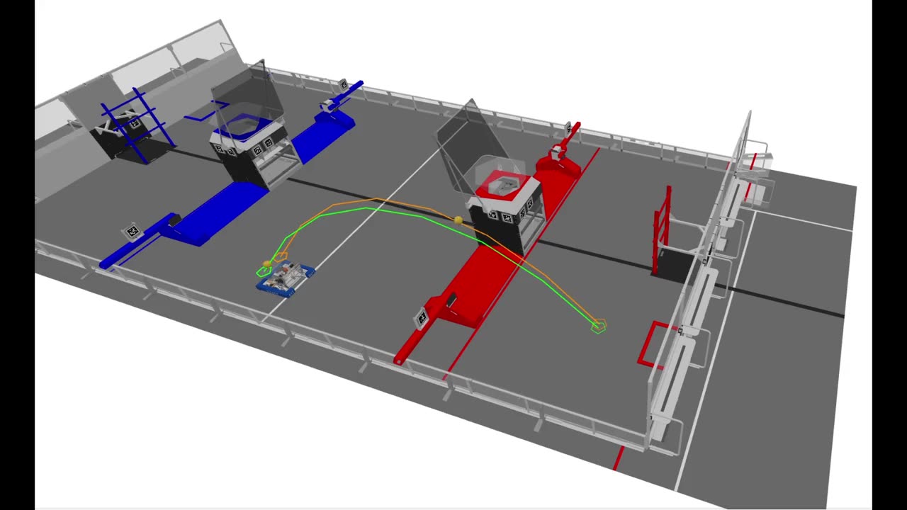
Field simulation of the 8393 robot lining up and taking a shot, with the projectile arc drawn live.
Featured above: Custom sim visualizing 3D trajectory and pose data to test physics ballistic solver
FIRST Robotics

Auto Aiming Mini Tank

Languages
Java
Tools
FTCLib, WPILib
When
2025–2026

Overview

For the 2025–2026 FTC & FRC season, I programmed a projectile-motion inspired shooting system to allow our robot to launch balls from anywhere on the field.

This project consists of 5 main components:

  1. Use the goal position, robot position, and a desired impact angle to calculate a 3D launch vector that will launch the ball into the goal
  2. Offset the launch vector by the robot velocity to allow shooting while moving
  3. Calculate a target turret and hood angle to compensate for deviations in actual exit speed
  4. Iteratively test the algorithm in simulation
  5. Design responsive & accurate control systems for the shooter, turret, and hood
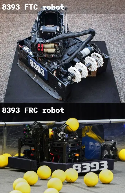
Two photographs labelled 8393 FTC robot and 8393 FRC robot. The FTC robot is a compact black chassis with a shooter assembly and white omni wheels; the FRC robot is a larger black drivebase on a competition field scattered with yellow game balls.

1 Computing desired 3D launch vector of ball

The parabolic curve of a projectile can be defined with 3 data points: a starting position, an ending position, and the angle of its velocity vector when at the ending position (this is a tunable constant which I call the impact angle). Using these 3 pieces of data, one can calculate the launch vector of the ball at any given robot position.

Show the math Hide the math

Let

vv
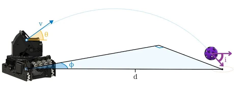
desired exit speed of the artifact
θ\theta
hood angle, measured from horizontal
ϕ\phi
turret angle
ii
desired impact angle — the angle of the ball’s velocity when it reaches the goal
hh
goal height minus exit height
dd
horizontal distance from the exit position to the goal
A side view of the shooter on the robot with the trajectory drawn as an arc to the goal. The exit velocity v leaves at hood angle θ above horizontal, the turret angle φ opens off the robot's heading across the horizontal distance d, and the impact angle i is marked at the ball where it meets the goal.

Projectile motion equations tell us that:

Position

Δx=v0t+12at2\Delta x = v_0 t + \tfrac{1}{2} a t^2 h=vsin⁡θ t−12gt2d=vcos⁡θ th = v\sin\theta\, t - \tfrac{1}{2} g t^2 \qquad d = v\cos\theta\, t t=dvcos⁡θt = \frac{d}{v\cos\theta} h=vsin⁡θ ⁣(dvcos⁡θ)−12g ⁣(dvcos⁡θ) ⁣2h = v\sin\theta\!\left(\frac{d}{v\cos\theta}\right) - \tfrac{1}{2} g\!\left(\frac{d}{v\cos\theta}\right)^{\!2} h=dtan⁡θ−gd22v2cos⁡2θh = d\tan\theta - \frac{g d^2}{2 v^2 \cos^2\theta} gd22v2cos⁡2θ=dtan⁡θ−h\frac{g d^2}{2 v^2 \cos^2\theta} = d\tan\theta - h

Velocity

Δv=at\Delta v = a t vx=vcos⁡θv_x = v\cos\theta vy=vsin⁡θ−gtv_y = v\sin\theta - g t i=tan⁡−1 ⁣(vyvx)i = \tan^{-1}\!\left(\frac{v_y}{v_x}\right) tan⁡i=vsin⁡θ−gtvcos⁡θ\tan i = \frac{v\sin\theta - g t}{v\cos\theta} tan⁡i=tan⁡θ−gtvcos⁡θ\tan i = \tan\theta - \frac{g t}{v\cos\theta}

Substituting the time of flight into the velocity relation, then folding in the position result:

tan⁡i=tan⁡θ−gvcos⁡θ ⁣(dvcos⁡θ)\tan i = \tan\theta - \frac{g}{v\cos\theta}\!\left(\frac{d}{v\cos\theta}\right) tan⁡i=tan⁡θ−gdv2cos⁡2θ\tan i = \tan\theta - \frac{g d}{v^2\cos^2\theta} tan⁡i=tan⁡θ−2 ⁣(dtan⁡θ−h)d\tan i = \tan\theta - \frac{2\!\left(d\tan\theta - h\right)}{d} tan⁡θ=tan⁡i+2 ⁣(dtan⁡θ−h)d\tan\theta = \tan i + \frac{2\!\left(d\tan\theta - h\right)}{d} tan⁡θ=tan⁡i+2tan⁡θ−2hd\tan\theta = \tan i + 2\tan\theta - \frac{2h}{d} tan⁡θ=2hd−tan⁡i\tan\theta = \frac{2h}{d} - \tan i

Ideal hood angle

θ=tan⁡−1 ⁣(2hd−tan⁡i)\theta = \tan^{-1}\!\left(\frac{2h}{d} - \tan i\right)

With the hood angle known, the same position result gives the speed it has to be fired at:

gd2v2cos⁡2θ=2 ⁣(dtan⁡θ−h)\frac{g d^2}{v^2\cos^2\theta} = 2\!\left(d\tan\theta - h\right) gd2cos⁡2θ ⁣(12 ⁣(dtan⁡θ−h))=v2\frac{g d^2}{\cos^2\theta}\!\left(\frac{1}{2\!\left(d\tan\theta - h\right)}\right) = v^2 v=gd22cos⁡2θ(dtan⁡θ−h)v = \sqrt{\frac{g d^2}{2\cos^2\theta\left(d\tan\theta - h\right)}}

Ideal exit speed

v=gd22cos⁡2θ(dtan⁡θ−h)v = \sqrt{\frac{g d^2}{2\cos^2\theta\left(d\tan\theta - h\right)}}

Ideal turret angle

ϕ=tan⁡−1 ⁣(ygoal−yrobotxgoal−xrobot)\phi = \tan^{-1}\!\left( \frac{y_{\text{goal}} - y_{\text{robot}}}{x_{\text{goal}} - x_{\text{robot}}} \right)

Constructing the 3D ball launch vector

v⃗ball=[vcos⁡θcos⁡ϕvcos⁡θsin⁡ϕvsin⁡θ]\vec{v}_{\text{ball}} = \begin{bmatrix} v\cos\theta\cos\phi \\[2pt] v\cos\theta\sin\phi \\[2pt] v\sin\theta \end{bmatrix}

2 Accounting for robot velocity

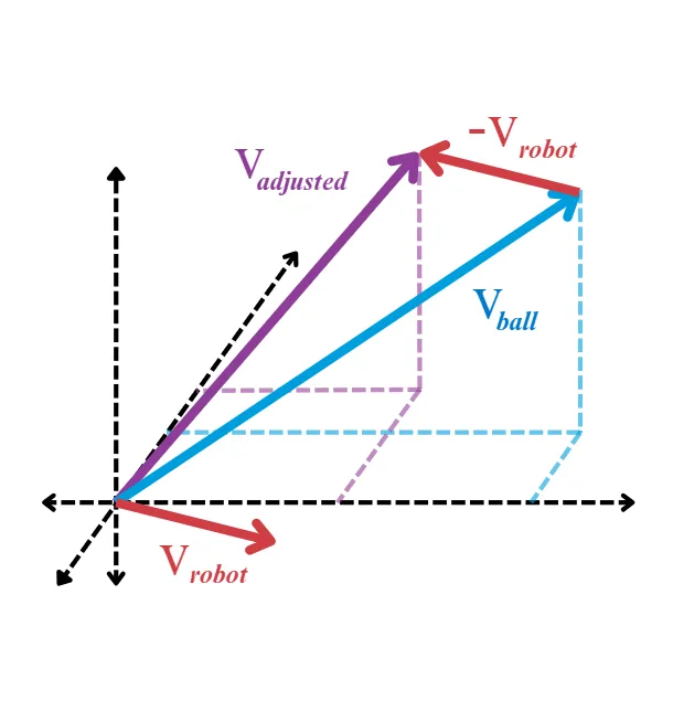
We also need a way to counteract the robot’s movement, because it will alter the trajectory of the ball. To do this, we can use vector subtraction and offset the previous 3D launch vector by the velocity at the ball’s exit position. Note: because the ball’s launch position is not guaranteed to be aligned with the robot’s axis of rotation, we also need to account for the tangential velocity created by rotation.

Show the math Hide the math

Assuming

v⃗cm\vec{v}_{cm}
robot velocity at center of mass (assumed axis of rotation)
ω⃗\vec{\omega}
robot angular velocity
r⃗\vec{r}
ball exit position relative to robot position
v⃗robot\vec{v}_{\text{robot}}
robot velocity at exit position of ball
v⃗ball\vec{v}_{\text{ball}}
desired 3D launch vector of ball
v⃗adjusted\vec{v}_{\text{adjusted}}
the actual launch vector we want to aim at
v⃗robot=v⃗cm+ω⃗×r⃗\vec{v}_{\text{robot}} = \vec{v}_{cm} + \vec{\omega} \times \vec{r}

Constructing the desired launch vector

v⃗adjusted+v⃗robot=v⃗ball\vec{v}_{\text{adjusted}} + \vec{v}_{\text{robot}} = \vec{v}_{\text{ball}} v⃗adjusted=v⃗ball−v⃗robot\vec{v}_{\text{adjusted}} = \vec{v}_{\text{ball}} - \vec{v}_{\text{robot}}

Finally, your target launch speed equals the length of this launch vector.

Target launch speed
∣v⃗adjusted∣=vadjusted,x 2+vadjusted,y 2+vadjusted,z 2\left|\vec{v}_{\text{adjusted}}\right| = \sqrt{ v_{\text{adjusted},x}^{\,2} + v_{\text{adjusted},y}^{\,2} + v_{\text{adjusted},z}^{\,2} }
A 3D vector diagram. The blue vector V_ball is the launch vector the ball needs; the red vector V_robot is the robot's own velocity along the floor, and its negative is added to the tip of V_ball; the purple vector V_adjusted is the result the shooter is actually commanded to.

3 Compensating for deviation in exit speed

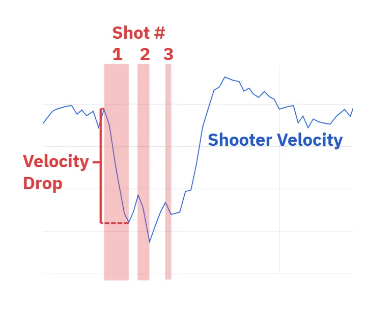
The Law of Conservation of Energy states that energy cannot be created. Therefore, when the shooter contacts the ball and the ball speeds up, the shooter wheel must slow down. Since the shooter wheel has lost some of its energy, it will transfer less energy to the next ball that is shot, decreasing shot accuracy.

To mitigate this problem, we can alter our hood angle — changing the arc of the trajectory — to compensate for the lower exit speed; and we can also alter our turret angle to ensure that we can still shoot on the move.

a: Deriving time of flight polynomial

Assuming

s⃗\vec{s}
possible launch vector
SS
current exit speed

We already know that:

s⃗+v⃗robot=v⃗ball\vec{s} + \vec{v}_{\text{robot}} = \vec{v}_{\text{ball}}

By component

sx+vrx=vbxs_x + v_{rx} = v_{bx} sy+vry=vbys_y + v_{ry} = v_{by} sz+vrz=vbzs_z + v_{rz} = v_{bz}

Displacement over the flight

vbx t=dxv_{bx}\,t = d_x vby t=dyv_{by}\,t = d_y vbz t−12gt2=dzv_{bz}\,t - \tfrac{1}{2} g t^2 = d_z
A telemetry plot of shooter wheel velocity over time. Three shots are marked as shaded bands; the wheel is running steadily before the first, and a labelled velocity drop takes it well below that level across the three shots before it recovers.
(sx+vrx)t=dx⟹sx=dxt−vrx\left(s_x + v_{rx}\right) t = d_x \quad\Longrightarrow\quad s_x = \frac{d_x}{t} - v_{rx} (sy+vry)t=dy⟹sy=dyt−vry\left(s_y + v_{ry}\right) t = d_y \quad\Longrightarrow\quad s_y = \frac{d_y}{t} - v_{ry} (sz+vrz)t−12gt2=dz⟹sz=dz+12gt2t−vrz\left(s_z + v_{rz}\right) t - \tfrac{1}{2} g t^2 = d_z \quad\Longrightarrow\quad s_z = \frac{d_z + \tfrac{1}{2} g t^2}{t} - v_{rz}

And assuming that you cannot instantaneously change your shooter speed:

S=sx 2+sy 2+sz 2S = \sqrt{s_x^{\,2} + s_y^{\,2} + s_z^{\,2}} S=(dxt−vrx) ⁣2+(dyt−vry) ⁣2+(dz+12gt2t−vrz) ⁣2S = \sqrt{ \left(\frac{d_x}{t} - v_{rx}\right)^{\!2} + \left(\frac{d_y}{t} - v_{ry}\right)^{\!2} + \left(\frac{d_z + \frac{1}{2} g t^2}{t} - v_{rz}\right)^{\!2} } S2=(dx 2t2−2dxvrxt+vrx 2)+(dy 2t2−2dyvryt+vry 2)+((dz+12gt2) ⁣2t2−2(dz+12gt2)vrzt+vrz 2)S^2 = \left(\frac{d_x^{\,2}}{t^2} - \frac{2 d_x v_{rx}}{t} + v_{rx}^{\,2}\right) + \left(\frac{d_y^{\,2}}{t^2} - \frac{2 d_y v_{ry}}{t} + v_{ry}^{\,2}\right) + \left( \frac{\left(d_z + \frac{1}{2} g t^2\right)^{\!2}}{t^2} - \frac{2\left(d_z + \frac{1}{2} g t^2\right) v_{rz}}{t} + v_{rz}^{\,2} \right)

Clearing the denominator:

S2t2=dx 2−2dxvrxt+vrx 2t2+dy 2−2dyvryt+vry 2t2+(dz+12gt2) ⁣2−2(dz+12gt2)vrzt+vrz 2t2\begin{aligned} S^2 t^2 ={}& d_x^{\,2} - 2 d_x v_{rx} t + v_{rx}^{\,2} t^2 \\[4pt] &+ d_y^{\,2} - 2 d_y v_{ry} t + v_{ry}^{\,2} t^2 \\[4pt] &+ \left(d_z + \tfrac{1}{2} g t^2\right)^{\!2} - 2\left(d_z + \tfrac{1}{2} g t^2\right) v_{rz} t + v_{rz}^{\,2} t^2 \end{aligned} S2t2=dx 2−2dxvrxt+vrx 2t2+dy 2−2dyvryt+vry 2t2+dz 2+dzgt2+14g2t4−2dzvrzt−gvrzt3+vrz 2t2\begin{aligned} S^2 t^2 ={}& d_x^{\,2} - 2 d_x v_{rx} t + v_{rx}^{\,2} t^2 \\[4pt] &+ d_y^{\,2} - 2 d_y v_{ry} t + v_{ry}^{\,2} t^2 \\[4pt] &+ d_z^{\,2} + d_z g t^2 + \tfrac{1}{4} g^2 t^4 - 2 d_z v_{rz} t - g v_{rz} t^3 + v_{rz}^{\,2} t^2 \end{aligned}

Collecting by power of tt leaves a quartic whose unknown is no longer the exit speed, but the time of flight:

Quartic in time of flight

0=∣d⃗∣2−2(d⃗⋅v⃗robot)t+(∣v⃗robot∣2−S2+gdz)t2−gvrzt3+14g2t40 = \left|\vec{d}\right|^2 - 2\left(\vec{d} \cdot \vec{v}_{\text{robot}}\right) t + \left(\left|\vec{v}_{\text{robot}}\right|^2 - S^2 + g d_z\right) t^2 - g v_{rz} t^3 + \tfrac{1}{4} g^2 t^4
b: Approximating the “best” flight time

Finding zeroes of time of flight polynomial

We want to find this function’s zeroes, because they represent all of the possible trajectories that we could take to compensate for an inaccurate launch speed. So I approximated the zeros using a two-stage search. First, the flight-time domain is discretized into low-resolution intervals to identify regions where the function crossed zero. These intervals were then refined with bisection, which repeatedly halves the interval until the root estimate achieved a maximum error of 10−310^{-3} seconds. At a maximum, the code could return 2 flight times (a low arc & a high arc shot). Returning 1 time of flight means the high and low arc shot converged (this trajectory minimizes launch speed). Returning 0 flight times signifies that the launch speed just dropped too much and there are no valid trajectories.

Recalculating the new launch vector

Let tallt_{\text{all}} be a list containing all real zeroes of that polynomial. For each candidate time t=tat = t_a :

v⃗ball(ta)=[dxtadytadz+12gta 2ta]\vec{v}_{\text{ball}}(t_a) = \begin{bmatrix} \dfrac{d_x}{t_a} \\[8pt] \dfrac{d_y}{t_a} \\[8pt] \dfrac{d_z + \frac{1}{2} g t_a^{\,2}}{t_a} \end{bmatrix} i(ta)=tan⁡−1 ⁣(vbz(ta)vbx(ta)2+vby(ta)2)i(t_a) = \tan^{-1}\!\left( \frac{v_{bz}(t_a)}{\sqrt{v_{bx}(t_a)^2 + v_{by}(t_a)^2}} \right)

Then pick the time of flight t=tft = t_f whose impact angle is closest to the desired impact angle.

c: Calculating compensated hood and turret angles

Plugging the time of flight into the launch vector equations

sx=dxtf−vrxs_x = \frac{d_x}{t_f} - v_{rx} sy=dytf−vrys_y = \frac{d_y}{t_f} - v_{ry} sz=dz+12gtf 2tf−vrzs_z = \frac{d_z + \frac{1}{2} g t_f^{\,2}}{t_f} - v_{rz}

Compensated hood angle

θ=tan⁡−1 ⁣(szsx 2+sy 2)\theta = \tan^{-1}\!\left( \frac{s_z}{\sqrt{s_x^{\,2} + s_y^{\,2}}} \right)

Compensated turret angle

ϕ=tan⁡−1 ⁣(sysx)\phi = \tan^{-1}\!\left(\frac{s_y}{s_x}\right)

4 Custom AdvantageScope Sim

The purpose of this simulation is to visualize 3D poses and trajectories, allowing me to extensively test my physics equations as well as robot behavior before deploying to the robot.

  • To visualize the shot arcs, I converted the launch vector into a parabolic equation, then generated points along the equation and drew lines connecting them.
  • To model the balls, I implemented Euler’s method and applied gravity to simulate a projectile.

5 Control System Design & Testing

For both FTC and FRC, our shooting system consists of 3 hardware components allowing us to accurately launch balls.

Choose a mechanism

Control System

Like all good things, I started with a PID. Then, to counteract the backEMF and friction in the motor, I added a feedforward velocity regression. And to communicate with the physics algorithm, I modeled a launch velocity to motor velocity conversion (see right). I also applied a time-invariant low pass filter to remove high frequency sensor noise.
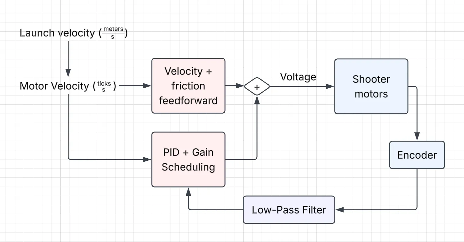
Block diagram of the shooter control system. Launch velocity in metres per second converts to a motor velocity in ticks per second, which splits into a velocity-and-friction feedforward and a gain-scheduled PID; the two sum into a voltage for the shooter motors, whose encoder feeds back through a low-pass filter into the PID.

System Identification

This regression relates a given motor velocity (x axis) to the ball’s launch velocity (y axis). Interestingly, a logarithmic curve best fit this data, showing that at higher speeds, more energy is lost in the shooter wheel-ball collision.
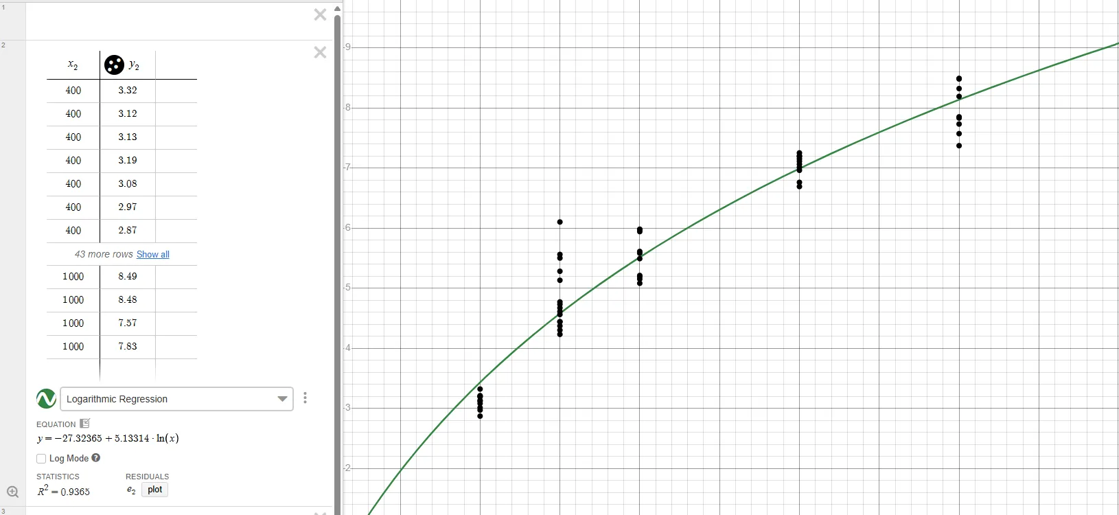
A Desmos logarithmic regression of ball exit speed against commanded motor velocity. Roughly fifty logged shots cluster in vertical stacks at each swept velocity from 400 up to 1000 ticks per second, with exit speeds from about 3 to 8.5 metres per second. The fit is y = −27.32 + 5.133·ln(x), R² = 0.9365.

Control System

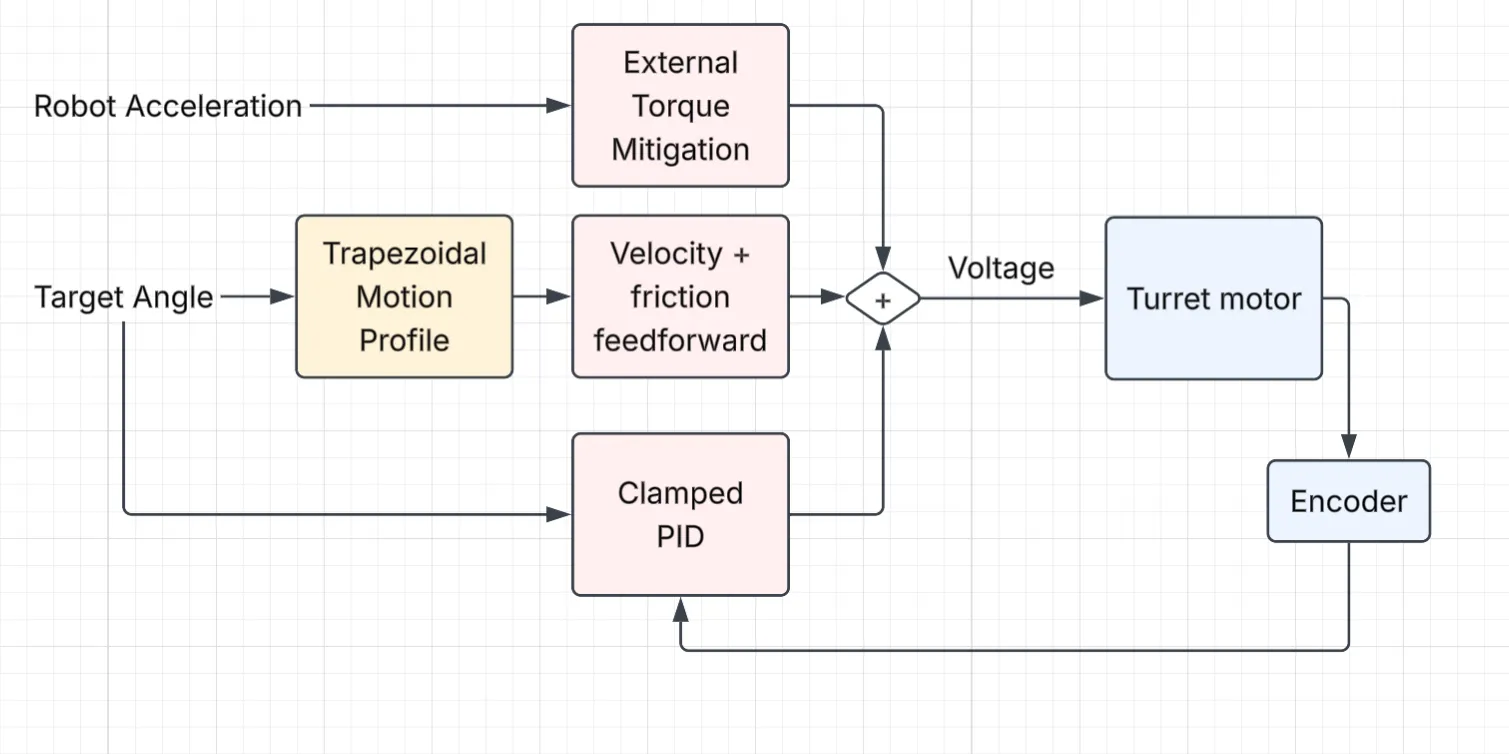
Similarly to the shooter, I also started with just a PID. Then I added a distance-based trapezoidal motion profiler using this equation:

vf2−vi2=2adv_f^2 - v_i^2 = 2ad

The output of the motion profiler is fed into a feedforward velocity regression, similar to that in the shooter (see right). And finally, because the shooter’s center of mass is not aligned with the turret’s axis of rotation, any robot acceleration will exert a torque on the turret. So I countered the external torque with this physics model:

V−=kT(a⃗robot×r⃗turret)V \mathrel{-}= k_T \left( \vec{a}_{\text{robot}} \times \vec{r}_{\text{turret}} \right)

VV = applied voltage, kTk_T = a tunable constant, a⃗robot\vec{a}_{\text{robot}} = robot acceleration, r⃗turret\vec{r}_{\text{turret}} = turret axis relative to robot axis

Block diagram of the turret control system. Target angle runs through a trapezoidal motion profile into a velocity-and-friction feedforward, and separately into a clamped PID; robot acceleration drives an external-torque mitigation term. All three sum into a voltage for the turret motor, whose encoder feeds back into the PID.

System Identification

Below is the feedforward turret velocity regression. The x axis is angular velocity (rad/s), and the y axis is applied voltage. The slope corresponds to kV and intercept corresponds to kS.
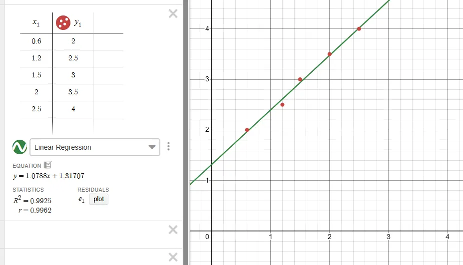
A Desmos linear regression from the turret velocity sweep: five measured points rising steadily from (0.6, 2) to (2.5, 4), fitted by y = 1.0788x + 1.317 with R² = 0.9925.

Control System

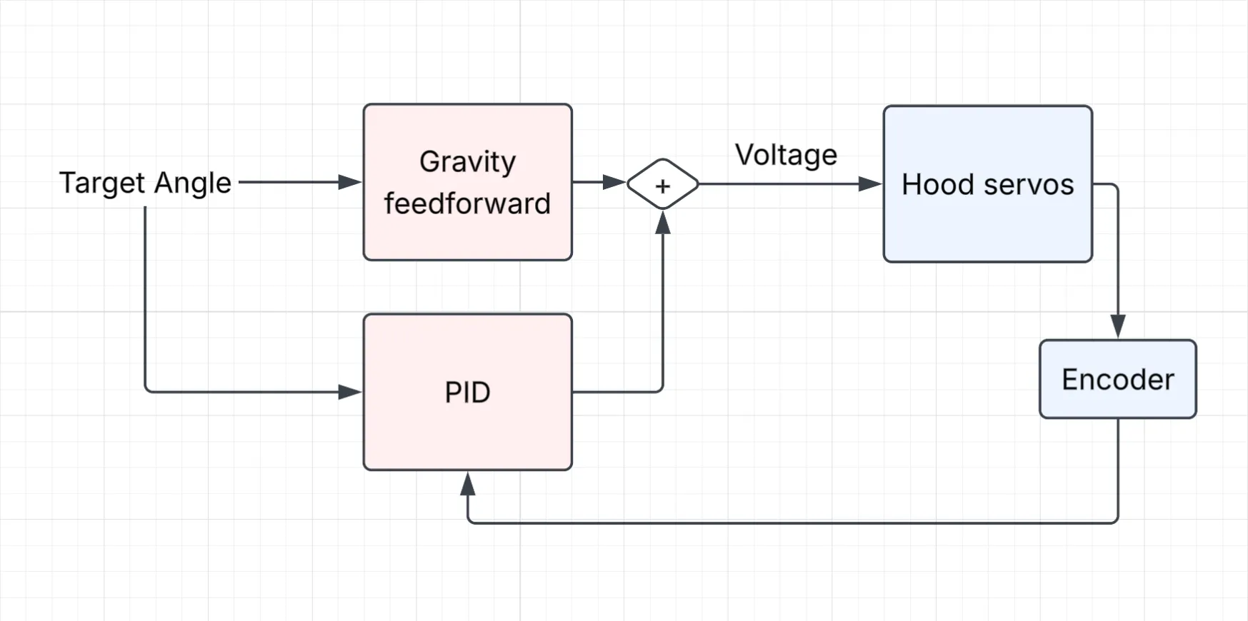
The hood control system is pretty simple; a PID with gravity feedforward modeled by

V+=kGcos⁡θV \mathrel{{+}{=}} k_G \cos\theta

VV = applied voltage, kGk_G = tunable constant, θ\theta = hood angle from horizontal

Block diagram of the hood control system. Target angle feeds a gravity feedforward and a PID in parallel; the two sum into a voltage for the hood servos, whose encoder feeds back into the PID.

System Identification

This regression maps hood encoder values to the actual angle from the horizontal. The x axis is encoders, and the y axis is angle (degrees).
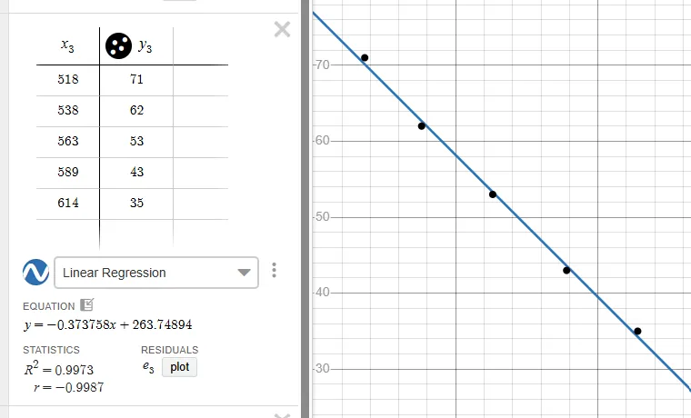
A Desmos linear regression tying the hood’s encoder reading to its measured angle: five points falling from (518, 71 degrees) to (614, 35 degrees), fitted by y = −0.3738x + 263.75 with R² = 0.9973.